Determining optimal store operating hours through historical transaction timestamp analysis

Every retail business is basically a system that generates revenue by converting customer demand into completed sales. The business cannot just extend its operating hours to increase its revenue – the correlation is not a simple linear function. Extending operating hours does not necessarily increase revenue proportionally, because additional operating hours also introduce additional labour and operating expenses. By contrast, shifting the existing operating window earlier or later keeps the total operating duration unchanged while changing which periods of customer activity are covered.

A retail business operates within a finite number of hours each day. Every business day therefore represents a fixed interval during which demand can be converted into sales. Selecting this interval is an optimization problem because changing its position within the day changes the amount of customer purchases while the business is open.

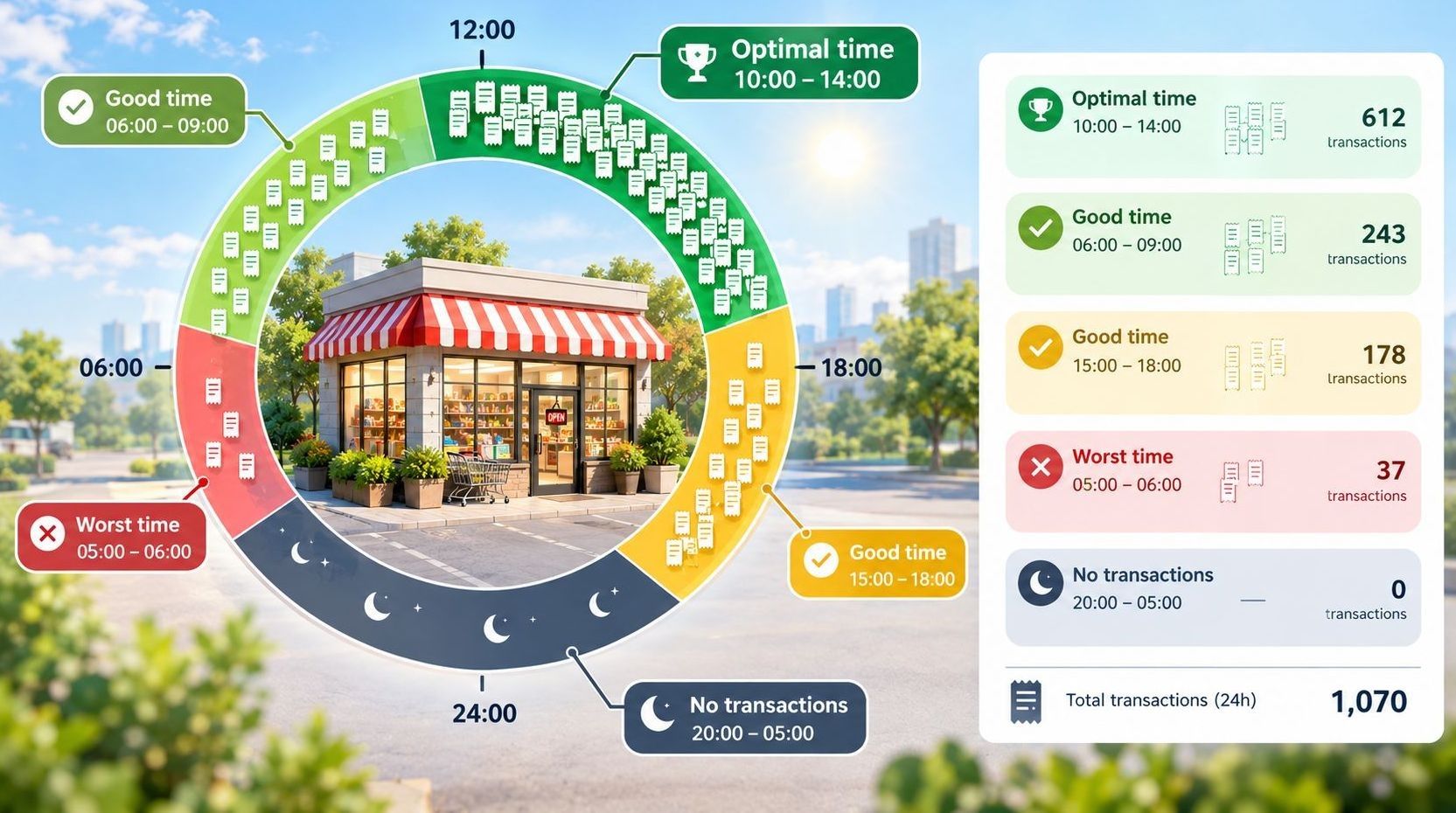
Given a fixed daily operating duration, the optimization task would be to determine the continuous operating window that contains the largest number of historically observed sales transactions.

For example, assume a retailer intends to operate for ten hours per day. Numerous operating schedules satisfy this requirement:

Schedule	Opening	Closing
A	07:00	17:00
B	08:00	18:00
C	09:00	19:00

Each schedule provides exactly the same operating duration. None receives additional trading time. The only variable is the position of the operating window within the day.

If customer purchasing activity is concentrated during early morning hours, an earlier opening schedule may include a greater number of completed transactions. Conversely, if purchasing activity continues into the evening, delaying both opening and closing may capture more sales while maintaining the same total operating time. The objective is therefore not to maximize the number of hours that the business remains open, but to determine where those hours should be positioned within the day.

This distinction is important because extending business hours and repositioning business hours are fundamentally different operational decisions. Extending operating hours increases staffing requirements, utility consumption and other operating costs. Repositioning operating hours keeps unchanged the daily duration and daily costs associated.

Why selection of the best operating hours may be counterintuitive

Operating hours are frequently established through convention rather than quantitative analysis. A schedule may remain unchanged because it has existed for many years, because nearby competitors operate during similar hours, or because management considers the selected timeframe reasonable. None of these approaches evaluates whether the chosen schedule captures the greatest proportion of observed customer demand.

Human judgement and feeling may not be the best tool for the task of selecting the period of the day with maximum number of sales. A store manager may remember unusually busy mornings, employees may recall mornings that appeared quiet, and customers may comment that they would prefer evening hours. These observations describe individual experiences rather than the complete historical distribution of sales.

The distinction between intuitive subjective evidence and observational data is fundamental in analytical decision making. Individual observations are influenced by recency, selective memory and exceptional events. Transaction databases record every completed sale using the same business process regardless of whether the day was exceptionally busy or exceptionally quiet. Consequently, historical transaction records provide a substantially more reliable basis for identifying recurring patterns of customer activity.

Several external factors influence when customers visit a retail store. Daily commuting patterns determine when employees travel to and from workplaces. Nearby schools influence pedestrian activity during morning arrival and afternoon dismissal. Industrial facilities often generate demand that follows production shifts rather than conventional office hours. Public transportation schedules affect customer accessibility, while shopping centres may experience concentrated activity immediately after surrounding businesses close for the day. These influences differ between locations and frequently change over time as local infrastructure and demographics evolve.

Because customer activity depends on numerous external variables, operating hours that perform well at one location cannot automatically be assumed optimal elsewhere. Even stores belonging to the same retail chain may exhibit different purchasing patterns despite selling similar products. Selecting operating hours by copying another location therefore substitutes one assumption for another without evaluating the historical evidence available for the store under consideration.

The objective of data analysis is not to replace managerial experience, but to supplement it with measurable evidence. Instead of asking whether a particular schedule appears reasonable, the analysis asks a more precise question: during which continuous time interval did completed sales historically occur most frequently?

Why historical sales transactions provide the real evidence

Every completed sale represents a recorded purchase event. Unlike customer surveys, manual observations or memory recollections, sales transactions are generated automatically during normal business operations. Their timestamps therefore provide an objective record of when recorded purchases occurred.

Enterprise resource planning systems such as SAP NetWeaver record the creation date and creation time of sales documents as part of routine transaction processing. Because these timestamps are created automatically, they provide a chronological history of when completed purchases occurred throughout the business day.

When accumulated over hundreds of operating days, these timestamps reveal the temporal distribution of completed customer purchases. They answer questions that cannot be answered reliably from memory alone.

For example:

• Do customers purchase more frequently immediately after opening or later in the morning?
• Does customer activity decline steadily throughout the afternoon or remain relatively constant until closing?
• Does a significant proportion of purchases occur shortly before closing time?
• Would delaying opening exclude many sales transactions?
• Would extending the operating window later into the evening capture a larger proportion of customer activity?

If customer activity is concentrated during early morning hours, opening later excludes transactions that historically occurred before the doors opened. Conversely, if customer activity extends into the evening, closing earlier excludes transactions that historically occurred later in the day. Since every operating schedule captures a different portion of daily customer activity, different schedules inevitably contain different numbers of completed transactions.

The optimization problem therefore becomes one of selecting the operating window that historically contained the greatest concentration of completed sales.

Formal definition of the optimization problem

This article treats one sales document as one transaction, provided that each sales document represents one completed sale in the source data. Every transaction contributes equally to the analysis regardless of the number of products purchased per transaction, or transaction value. Consequently, the optimization criterion is the total number of sales transactions contained within a candidate operating window.

This baseline assumption emerges from the data source peculiarities. SAP’s VBAP table contains sales documents, with each representing an item sold, rather than unique sales transactions.

Alternative optimization criteria are possible. A retailer might instead choose to maximize total revenue, gross profit, average basket value or units sold. Those objectives require additional information beyond transaction timestamps and therefore fall outside the scope of the available dataset.

The optimization problem can therefore be stated as follows:

Determine the continuous operating interval of fixed duration that contains the greatest number of completed sales transactions recorded during the observation period.

Several characteristics of this formulation deserve attention.

• The operating duration is fixed throughout the optimization.
• Every candidate schedule spans exactly the same number of hours.
• The only variable is the opening time.
• The closing time changes automatically because the operating duration remains constant.
• Every completed transaction contributes one observation.
• The schedule containing the largest number of observations is considered the optimal solution under the chosen optimization criterion.

Restricting the problem in this manner improves the scientific validity of the analysis. Every conclusion remains directly traceable to recorded observations. Should additional business information become available in the future, such as transaction value, gross margin or labour costs, alternative optimization criteria may be investigated using the same analytical framework.

Observations data source

The analysis is based on historical sales transactions exported from an SAP NetWeaver system. Each record represents a completed sale and contains the timestamp at which the transaction was registered. No customer demographics, product information, or financial metrics are required for the objective considered in this study. The timestamp alone is sufficient because the optimization criterion depends exclusively on the temporal distribution of completed sales.

The analysis assumes that the historical observation period spans several years. A long observation period reduces the influence of short-term fluctuations caused by promotions, holidays, supply shortages, weather conditions, or other isolated events. Instead of describing the activity of a particular week or month, the resulting distribution reflects the purchasing behaviour observed at the store.

The objective is intentionally limited. The analysis identifies the operating interval that historically contained the largest number of completed sales.

Limiting the data timespan to make it more representative

Although the store’s SAP database contains records dating back to 2010, including the entire history would reduce the relevance of the analysis. Customer purchasing behaviour is not stationary over long periods. Changes in population, consumer habits, surrounding neighbor businesses, inflation, online shopping, and the structural effects following the COVID-19 pandemic have major altering power over shopping patterns. Consequently, transaction records from fifteen years ago should not be given equal weight when selecting business hours for current operations.

Rather than maximizing the number of observations, the objective is to analyze customer behaviour that is representative of present-day conditions. Restricting the dataset to the most recent years provides a better balance between statistical reliability and business relevance. In this study, only sales recorded during 2025 and 2026 are included in the analysis.

How to export transaction timestamps from SAP NetWeaver

SAP NetWeaver stores sales order information across multiple tables, each serving a different purpose within the transactional model. Since the analysis requires precise registration timestamps together with filtering by plant, data must be extracted in two stages.

The first stage utilizes the transaction SE16N, which provides direct access to SAP database tables. This T-code allows access to the item table VBAP (sales document item data). The data contained within this table should be filtered by the WERKS field, allowing records to be filtered for a specific store (in SAP this is often regarded to as a plant). Also, restricting the observation period can be achieved using the creation date field (ERDAT).

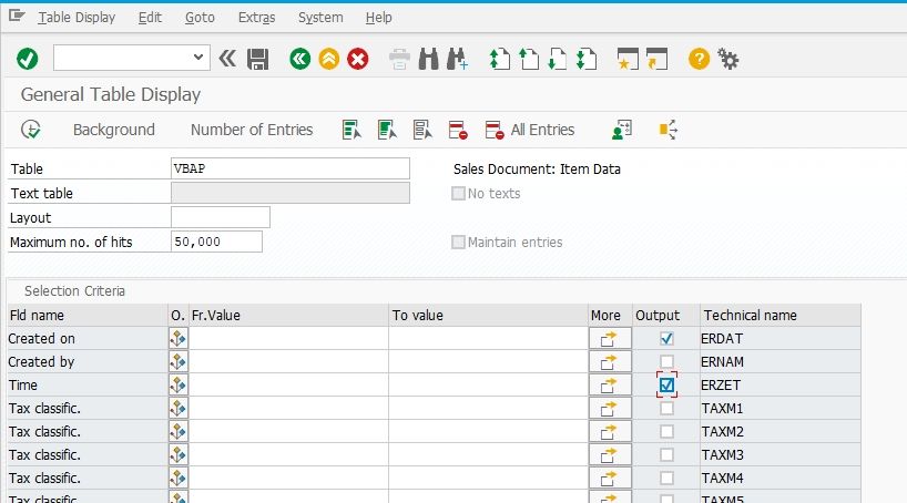
Since the optimization problem concerns the distribution of sales throughout the day, timestamps with minute-level precision are required. To export timestamps with this level of time precision, verify the time field (ERZET) is selected.

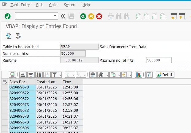
These fields are exported to Microsoft Excel, where the remaining preprocessing and analytical steps are performed.

Analyzing the dataset in Excel

The exported timestamps contain second-level precision, which obscures recurring demand patterns. To get a clear view of the temporal distribution, individual timestamps should be aggregated into fixed-length intervals. The interval length determines the balance between temporal resolution and statistical stability. Extremely short intervals, such as one minute, produce highly variable counts, conversely, hourly aggregation smooths the data, but risk hiding local demand peaks.

A twenty-minute interval provides a practical compromise. It is purely an analytical design choice, which is finer than 30, 40, 60 minutes without creating the workload of 10- or 5-minute intervals. Each hour is divided into three equal segments, allowing demand to be evaluated at 00, 20, and 40 minutes past the hour. The timestamps exported from SAP database are rounded downward to the nearest twenty-minute boundary.

In Microsoft Excel, the transformation is performed using the following formula:

=TEXT(FLOOR(B2 + TIME(1,0,0), TIME(0,20,0)), "HH:MM")

where column B contains the original SAP timestamp.

The formula performs three operations sequentially:

1. adds the required hour offset, since SAP stores time of its server, not the local time of the retail store (this matters for countries with several time zones, and international sales). In this dataset, the SAP timestamp required a one-hour correction to correspond to the store's local time;
2. rounds the adjusted timestamp downward to the nearest twenty-minute boundary using FLOOR command;
3. converts the rounded value into a formatted time label suitable for grouping within Excel Pivot Tables.

Example: a transaction registered at 15:37 is therefore assigned to the 15:20 interval, while a transaction occurring at 15:58 becomes part of the 15:40 interval.

Grouping transactions in this manner converts individual sales into a frequency distribution suitable for aggregation, and subsequent visualization, offering easy to understand trend for optimisation. The transformation also ensures that every sale belongs to exactly one interval, preventing duplication or ambiguity during later calculations.

How the exported dataset was analyzed in Excel

Step 1. Open the exported dataset

Open the spreadsheet exported from SAP NetWeaver. Verify that the date and time columns are recognized by Excel as a date rather than plain text. A simple verification consists of changing the cell format. If Excel allows the date to be displayed in different formats (for example, 09-Jun-2025 or 2025-06-09), the value has been imported correctly. If changing the format has no effect, the column contains text and should first be converted into proper dates.

Step 2. Create a 20-minute interval column

Insert a new column named Time Interval. If the timestamps obtained from the SAP database are stored in column B, enter the following formula into the first data row.

=TEXT(FLOOR(B2+TIME(1,0,0),TIME(0,20,0)),"HH:MM")

The formula performs three operations:

• applies the required one-hour correction (modify the correction accordingly to the time zone difference of the store and SAP server),
• rounds every timestamp downward to the nearest 20-minute interval (08:49:59 → 08:40)
• keeps the result in a human readable format of HOURS:MINUTES.

Copy the formula to every remaining row to get a dataset that contains a categorical variable representing the twenty-minute interval during which each sale occurred.

Step 3. Filter the observation period

Start with the exported Excel data and apply a filter to the column that contains full date of a transaction. In our example this is Created on column.

1. Select the entire dataset, including the column headers.
2. Click on the arrow near the header of the Created on column.
3. Set the filter for the date range to include records from 01/01/2025 through 31/12/2026.

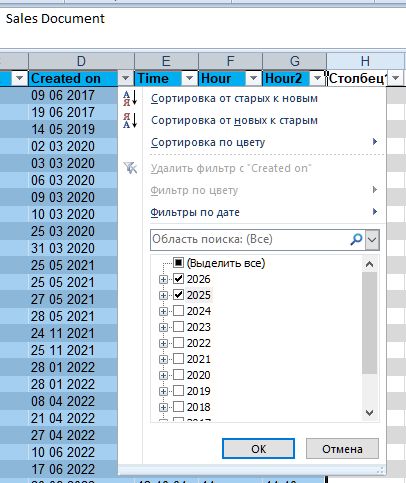
The important point is that the filter must be applied to the actual date values, not merely to displayed text. If Excel recognises Created on as a date, the filter will provide date-based conditions such as Greater Than or Equal To and Less Than or Equal To.

Because the current date may be earlier than the last day of the desired time range, there may naturally be no records for the remaining part of the last year within the filter. The upper boundary simply defines the intended analysis period; Excel will use whatever observations actually exist up to the latest available date.

Step 4. Analyze data using Pivot Table

Excel's Pivot Table is sufficient for this aggregation and avoids modifying the underlying transaction records.

1. Select the exported data

Click any cell inside the exported dataset. If the data has been converted to an Excel Table, selecting one cell is sufficient because Excel will recognize the complete table automatically. Otherwise, select the complete range containing the transaction records, including the column headers.

2. Insert the PivotTable

With the dataset selected, go to Insert → PivotTable. Excel will display the PivotTable creation dialog. Confirm that the selected table or range contains the complete transaction dataset. Select New Worksheet as the destination and click OK.

Excel will create an empty PivotTable and display the PivotTable Fields panel. The panel contains the fields from the exported SAP data and four areas into which fields can be placed: Filters, Columns, Rows and Values.

3. Put the 20-minute time field into Rows

The field used for the final distribution should represent the 20-minute interval assigned to each transaction. If this field has already been created, use it here. In our dataset this is Hour2 column.

Drag the 20-minute time field into the Rows area.

The PivotTable will then create one row for each time interval occurring in the source data. The ordering should be chronological, from 00:00 through 23:40. If Excel sorts the intervals alphabetically rather than chronologically, the underlying time values are probably stored as text and should be converted to actual Excel time values before proceeding.

4. Put the sales transactions into Values

Drag Sales Document into the Values area. The PivotTable should now contain two columns: Time interval and Count of Sales Document.

The PivotTable may omit intervals with zero transactions. This does not affect the moving-window calculation, because the calculation evaluates the actual time values in the distribution and treats absent intervals as having zero transactions.

Before using the distribution for optimization, verify that the PivotTable represents the intended dataset. The sum of all interval counts should equal the number of transaction records included after applying the date filter.

This check is useful because an apparently plausible distribution can still be based on an incorrectly filtered source range, an incomplete PivotTable source, or an inappropriate value calculation. The total count provides a simple reconciliation between the raw transaction dataset and the aggregated distribution.

7. The resulting distribution

After these steps, the raw SAP transaction data has been reduced to a compact daily distribution:

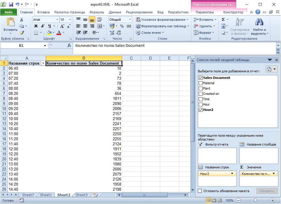
Preserve this table as the input to the optimization. The table describes the historical distribution of transactions; the optimization is performed in the next stage by evaluating consecutive groups of intervals corresponding to the proposed operating duration.

The next step is to define the candidate operating duration and slide a window of that duration across the 20-minute distribution.

Select the optimal business operating time window

The PivotTable now provides the observed transaction distribution in 20-minute intervals. The next step is to transform this distribution into an optimisation problem. The next step is to determine where a fixed operating period should be placed to capture the largest possible number of transactions.

The problem can be expressed as a moving-window optimisation. A window representing the required operating duration is moved through the time distribution, and the transaction counts within each candidate window are summed. The window with the highest total is the optimal operating period for the selected duration.

The objective is now to make Excel automatically answer this question:

Step 1: Enter the desired operating duration

Choose an empty cell, for example D1, and enter the header for operating duration of the store in hours. In E1, enter the desired duration. For example: 8. The value in E1 is the only parameter that will need to be changed when testing different operating durations.

Step 2: Convert the duration into 20-minute intervals

In D2, enter: Number of 20-minute intervals. In E2, enter: =E1*3

For an eight-hour operating period, Excel returns 24, because eight hours contain twenty four 20-minute intervals.

Step 3: Create the candidate start-time column

In D4, enter: Candidate start. In E4, enter: Candidate end. In F4, enter: Transactions in window.

Now copy the time intervals from the PivotTable into column D, or simply reference them.

In D5, enter: =A2

Then copy the formula down through all time slots, in this case up to D21. Cell D21 corresponds to the final valid window start time of 12:00. Later start times would extend beyond the available observation range and are therefore not considered.

Step 4: Calculate the end time automatically

In E5, enter: =D5+TIME($E$1,0,0)

In case the formula results in a decimal fraction, convert cells into Time format. Then copy the formula down through cell E21.

Excel now calculates the end of every candidate window automatically.

Step 5: Calculate the amount of transactions inside every time window

In cell F5, enter formula: =SUMPRODUCT((TIMEVALUE($A$2:$A$39)>=D5)*(TIMEVALUE($A$2:$A$39)Then copy the formula down.

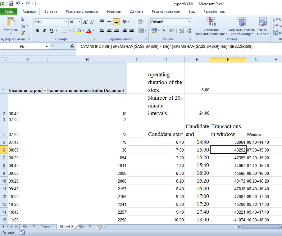
Step 6: Identify the maximum transaction count

In cell D44, enter: Maximum transactions. Verify the cell E44 is converted to Number format, and enter: =MAX(F5:F21)

This returns the largest transaction total among all candidate windows.

Step 7: Visualizing the sales data to see the optimal business operating time window

The moving-window calculation can be easier to understand in the graphic chart format.

In the calculation table, the start time is stored in column D and the end time in column E, while column F contains the calculated number of transactions for each candidate window. Add a new column, G, with the heading Window. In cell G7, enter the following formula =TEXT(D7,"hh:mm")&"–"&TEXT(E7,"hh:mm")

Copy the formula down through all candidate windows.

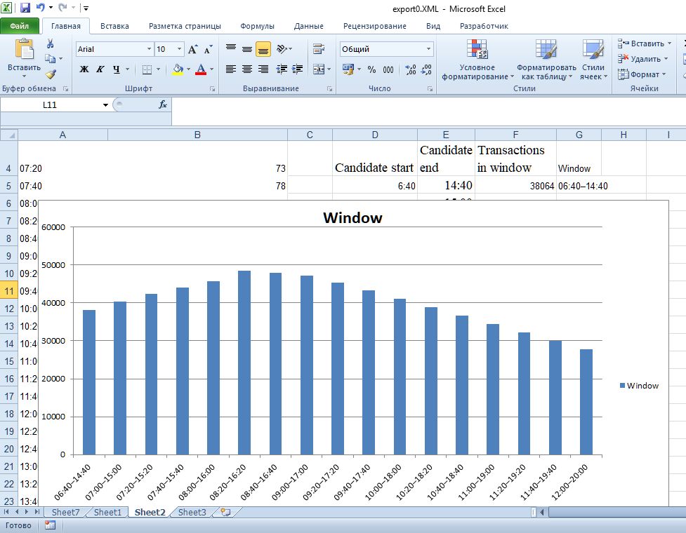
To create the chart, select the Window column together with the corresponding Transactions in window column. Then choose: Insert → Charts → Column or Bar Chart → 2-D Column → Clustered Column.

The horizontal axis will contain the operating time windows, while the vertical axis will show the total number of transactions captured by each window.

The resulting chart provides a direct visual representation of the optimization landscape. Each column represents one possible operating schedule, and its height represents the number of transactions that would fall inside that schedule. The highest column therefore corresponds to the optimal window under the defined objective of a period containing the maximum number of transactions.

Final summary

The typical workday usually has a fixed 8-hour operating period. But there is no obvious reason why those 8 hours should begin at one particular time rather than another. Often, the operating time slot is selected based on management's subjective preference. Alas, a poorly chosen timeframe can leave a significant part of customer activity outside the selected hours, while another timeframe of exactly the same duration can capture considerably more of it.

The finished worksheet performs the entire optimisation through one chain of calculations to determine which operating time slot within the analysed day contains the largest number of recorded sales transactions.

• the SAP NetWeaver export provides the historical transaction timestamps;
• the Excel PivotTable aggregates transactions into 20-minute intervals;
• the candidate start and end times define each possible 8-hour operating window;
• the calculation formula sums the transactions falling within each window;
• the candidate windows are ranked by their total transaction count;
• the maximum identifies the operating period containing the largest number of transactions; and
• the visual chart of transaction totals distribution across time slots allows the transaction volume of different operating periods to be compared intuitively.

Once this has been established, the manager no longer needs to rely solely on subjective intuition when selecting an operating schedule for a retail store. The decision can instead be supported by the historical transaction data and a systematic comparison of the available operating periods.

The resulting schedule should be interpreted specifically as the window with the highest observed transaction count in the analysed data. It does not, by itself, establish that this schedule produces the highest profit or lowest operating cost. Those conclusions would require additional data such as transaction values, margins, staffing costs, and other operating expenses.

This article provides a simple and reproducible way to evaluate operating hours using historical transaction data. Rather than selecting a schedule based on general assumptions about customer behaviour, the analyst can compare the available operating windows quantitatively and select the one supported by the observed transaction distribution.